import numpy as np
import matplotlib.pyplot as plt
import cvxpy as cp
import jax
from jax import numpy as jnp, grad, jit
from scipy.optimize import minimize_scalar
import time
from sklearn.preprocessing import StandardScaler
from sklearn.datasets import make_classification
from sklearn.model_selection import train_test_split
# Set a random seed for reproducibility
jax.config.update("jax_enable_x64", True)
def fix_seed(seed=228):
np.random.seed(seed)
jax.random.PRNGKey(seed)
# Define the logistic loss function
@jit
def logistic_loss(w, X, y):
m = len(X)
z = X @ w
# Numerically stable version of logistic loss
loss = jnp.mean(jnp.logaddexp(0, -y * z))
return loss
# Compute predictions and accuracy for binary classification
@jit
def compute_accuracy(w, X, y):
predictions = jnp.sign(X @ w)
return jnp.mean(predictions == y)
# Compute the optimal solution using CVXPY
def compute_optimal(X, y, lam):
m, n = X.shape
# Define the variable for weights
w = cp.Variable(n)
# Construct the objective: logistic loss + L1 regularization
z = X @ w
# CVXPY implementation of logistic loss
logistic = cp.sum(cp.logistic(cp.multiply(-y, z))) / m
l1_reg = lam * cp.norm1(w)
# Total loss
loss = logistic + l1_reg
# Define the problem
problem = cp.Problem(cp.Minimize(loss))
# Solve the problem
problem.solve()
# Extract the optimal weights and minimum loss
w_star = w.value
f_star = problem.value
return w_star, f_star
# Generate synthetic classification problem
def generate_problem(params):
fix_seed()
m = params["m"] # number of samples
n = params["n"] # number of features
# Generate a binary classification dataset
X, y = make_classification(
n_samples=m,
n_features=n,
n_informative=int(n * 0.8),
n_redundant=int(n * 0.1),
n_repeated=0,
n_classes=2,
random_state=228,
class_sep=2.0
)
# Convert labels to -1, 1 for logistic regression
y = 2 * y - 1
# Split into train and test sets
X_train, X_test, y_train, y_test = train_test_split(X, y, test_size=0.2, random_state=228)
# Standardize features
scaler = StandardScaler()
X_train = scaler.fit_transform(X_train)
X_test = scaler.transform(X_test)
# Verify the actual condition number
H = X_train.T @ X_train / len(X_train)
actual_eigenvalues = np.linalg.eigvalsh(H)
actual_mu = np.min(actual_eigenvalues)
actual_L = np.max(actual_eigenvalues)
mu = params.get("mu", 0.0)
L = params.get("L", 10.0)
condition_str = "infinite" if mu == 0 else f"{L/mu:.6f}"
print(f"Requested spectrum bounds: mu={mu}, L={L}, condition number={condition_str}")
print(f"Actual spectrum bounds: mu={actual_mu:.6f}, L={actual_L:.6f}, condition number={actual_L/actual_mu:.6f}")
return X_train, y_train, X_test, y_test
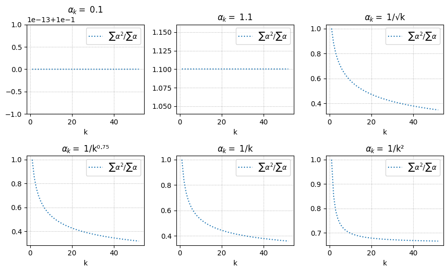
# Helper function to create a 1/sqrt(k) learning rate strategy
def create_1_over_sqrt_k_lr(alpha):
"""
Creates a learning rate function that returns alpha/sqrt(k) where k is the iteration number.
Args:
alpha: Scaling factor for the learning rate
Returns:
A function that takes an iteration number k and returns alpha/sqrt(k)
"""
def one_over_sqrt_k_lr(k):
# Avoid division by zero for k=0
k_safe = max(k, 1)
return alpha / (k_safe**0.5)
return one_over_sqrt_k_lr
# Helper function to create a 1/k learning rate strategy
def create_1_over_k_lr(alpha):
"""
Creates a learning rate function that returns alpha/k where k is the iteration number.
Args:
alpha: Scaling factor for the learning rate
Returns:
A function that takes an iteration number k and returns alpha/k
"""
def one_over_k_lr(k):
# Avoid division by zero for k=0
k_safe = max(k, 1)
return alpha / k_safe
return one_over_k_lr
# Subgradient descent method
def subgradient_descent(w_0, X_train, y_train, X_test, y_test, learning_rate, num_iters, lam):
fix_seed()
trajectory = [w_0]
times = [0]
train_accuracies = [compute_accuracy(w_0, X_train, y_train)]
test_accuracies = [compute_accuracy(w_0, X_test, y_test)]
w = w_0
f = lambda w: logistic_loss(w, X_train, y_train)
iter_start = time.time()
for i in range(num_iters):
# Determine the current learning rate
if callable(learning_rate):
# If learning_rate is a function, call it with the current iteration
current_lr = learning_rate(i+1)
else:
# Otherwise, use the constant learning rate
current_lr = learning_rate
grad_val = grad(f)(w)
subgrad_val = grad_val + lam * jnp.sign(w)
w = w - current_lr * subgrad_val
iter_time = time.time()
trajectory.append(w)
times.append(iter_time - iter_start)
train_accuracies.append(compute_accuracy(w, X_train, y_train))
test_accuracies.append(compute_accuracy(w, X_test, y_test))
return trajectory, times, train_accuracies, test_accuracies
# Soft thresholding operator for proximal gradient method
def soft_thresholding(x, kappa):
return jnp.sign(x) * jnp.maximum(jnp.abs(x) - kappa, 0)
# Proximal gradient method (ISTA)
def proximal_gradient_method(w_0, X_train, y_train, X_test, y_test, learning_rate, num_iters, lam):
trajectory = [w_0]
times = [0]
train_accuracies = [compute_accuracy(w_0, X_train, y_train)]
test_accuracies = [compute_accuracy(w_0, X_test, y_test)]
w = w_0
f = lambda w: logistic_loss(w, X_train, y_train)
iter_start = time.time()
for i in range(num_iters):
grad_val = grad(f)(w)
w = soft_thresholding(w - learning_rate * grad_val, learning_rate * lam)
iter_time = time.time()
trajectory.append(w)
times.append(iter_time - iter_start)
train_accuracies.append(compute_accuracy(w, X_train, y_train))
test_accuracies.append(compute_accuracy(w, X_test, y_test))
return trajectory, times, train_accuracies, test_accuracies
# Accelerated proximal gradient method (FISTA)
def accelerated_proximal_gradient(w_0, X_train, y_train, X_test, y_test, learning_rate, num_iters, lam):
trajectory = [w_0]
times = [0]
train_accuracies = [compute_accuracy(w_0, X_train, y_train)]
test_accuracies = [compute_accuracy(w_0, X_test, y_test)]
w = w_0
z = w_0
t = 1
f = lambda w: logistic_loss(w, X_train, y_train)
iter_start = time.time()
for i in range(num_iters):
grad_val = grad(f)(z)
w_next = soft_thresholding(z - learning_rate * grad_val, learning_rate * lam)
t_next = (1 + jnp.sqrt(1 + 4 * t**2)) / 2
z = w_next + ((t - 1) / t_next) * (w_next - w)
w = w_next
t = t_next
iter_time = time.time()
trajectory.append(w)
times.append(iter_time - iter_start)
train_accuracies.append(compute_accuracy(w, X_train, y_train))
test_accuracies.append(compute_accuracy(w, X_test, y_test))
return trajectory, times, train_accuracies, test_accuracies
# Compute metrics
def compute_metrics(trajectory, x_star, f_star, train_accuracies, test_accuracies, times, X_train, y_train, lam):
f = lambda w: logistic_loss(w, X_train, y_train) + lam * jnp.sum(jnp.abs(w))
metrics = {
"f_gap": [jnp.abs(f(x) - f_star) for x in trajectory],
"x_gap": [jnp.linalg.norm(x - x_star) for x in trajectory],
"train_accuracy": train_accuracies,
"test_accuracy": test_accuracies,
"time": times,
"sparsity": [jnp.mean(jnp.abs(x) < 1e-5) for x in trajectory]
}
return metrics
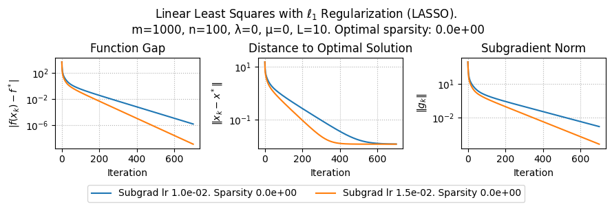
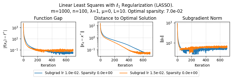
def run_experiments(params):
lam = params["lambda"]
methods = params["methods"]
results = {}
X_train, y_train, X_test, y_test = generate_problem(params)
n_features = X_train.shape[1]
# Initialize with zeros
x_0 = jax.random.normal(jax.random.PRNGKey(0), (n_features, ))
# Compute optimal solution
x_star, f_star = compute_optimal(X_train, y_train, lam)
optimal_sparsity = np.mean(np.abs(x_star) < 1e-5)
print(f"Optimal solution sparsity: {optimal_sparsity:.2e}")
params["optimal_sparsity"] = optimal_sparsity
print(f"Optimal train accuracy: {compute_accuracy(x_star, X_train, y_train):.4f}")
print(f"Optimal test accuracy: {compute_accuracy(x_star, X_test, y_test):.4f}")
for method in methods:
if method["method"] == "Subgrad":
learning_rate = method["learning_rate"]
iterations = method["iterations"]
# Handle different learning rate strategies
if isinstance(learning_rate, (int, float)):
# Constant learning rate
lr_label = f" lr {learning_rate:.1e}"
elif callable(learning_rate):
# Try to determine the type of learning rate scheduler
if hasattr(learning_rate, "__name__"):
if learning_rate.__name__ == "one_over_k_lr":
# 1/k learning rate
alpha = learning_rate.__closure__[0].cell_contents
lr_label = f" lr α/k (α={alpha:.1e})"
elif learning_rate.__name__ == "one_over_sqrt_k_lr":
# 1/sqrt(k) learning rate
alpha = learning_rate.__closure__[0].cell_contents
lr_label = f" lr α/√k (α={alpha:.1e})"
else:
lr_label = " lr custom"
elif hasattr(learning_rate, "__closure__") and learning_rate.__closure__:
# Try to extract the alpha value from the closure
try:
alpha = learning_rate.__closure__[0].cell_contents
# Check the function body to determine if it's 1/k or 1/sqrt(k)
func_code = learning_rate.__code__.co_consts
if any("k**0.5" in str(const) for const in func_code if isinstance(const, str)):
lr_label = f" lr α/√k (α={alpha:.1e})"
elif any("k**1" in str(const) for const in func_code if isinstance(const, str)):
lr_label = f" lr α/k (α={alpha:.1e})"
else:
lr_label = " lr custom"
except:
lr_label = " lr custom"
else:
lr_label = " lr custom"
else:
# Default to unknown if not recognized
lr_label = " lr unknown"
trajectory, times, train_accuracies, test_accuracies = subgradient_descent(
x_0, X_train, y_train, X_test, y_test, learning_rate, iterations, lam
)
label = method["method"] + lr_label
results[label] = compute_metrics(
trajectory, x_star, f_star, train_accuracies, test_accuracies, times, X_train, y_train, lam
)
elif method["method"] == "Proximal":
learning_rate = method["learning_rate"]
iterations = method["iterations"]
trajectory, times, train_accuracies, test_accuracies = proximal_gradient_method(
x_0, X_train, y_train, X_test, y_test, learning_rate, iterations, lam
)
label = method["method"] + f" lr {learning_rate:.1e}"
results[label] = compute_metrics(
trajectory, x_star, f_star, train_accuracies, test_accuracies, times, X_train, y_train, lam
)
elif method["method"] == "FISTA":
learning_rate = method["learning_rate"]
iterations = method["iterations"]
trajectory, times, train_accuracies, test_accuracies = accelerated_proximal_gradient(
x_0, X_train, y_train, X_test, y_test, learning_rate, iterations, lam
)
label = method["method"] + f" lr {learning_rate:.1e}"
results[label] = compute_metrics(
trajectory, x_star, f_star, train_accuracies, test_accuracies, times, X_train, y_train, lam
)
return results, params
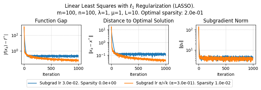
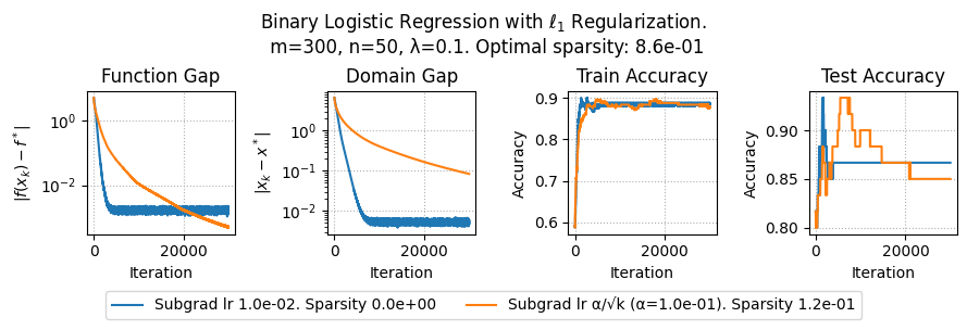
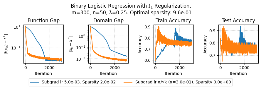
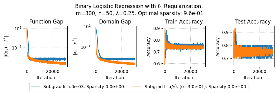
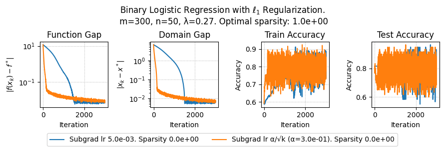
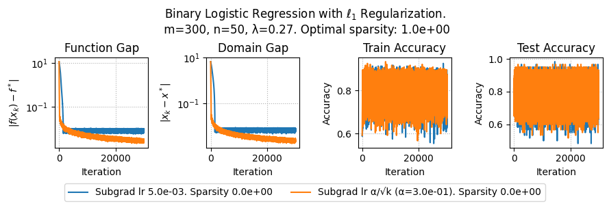
def plot_results(results, params):
plt.figure(figsize=(9, 3))
lam = params["lambda"]
plt.suptitle(f"Binary Logistic Regression with $\ell_1$ Regularization.\n m={params['m']}, n={params['n']}, λ={lam}. Optimal sparsity: {params['optimal_sparsity']:.1e}")
# Plot function gap vs iterations
plt.subplot(1, 4, 1)
for method, metrics in results.items():
plt.plot(metrics['f_gap'], label=method + f". Sparsity {metrics['sparsity'][-1]:.1e}")
plt.xlabel('Iteration')
plt.ylabel(r'$|f(x_k) - f^*|$')
plt.yscale('log')
plt.grid(linestyle=":")
plt.title('Function Gap')
plt.subplot(1, 4, 2)
for method, metrics in results.items():
plt.plot(metrics['x_gap'])
plt.xlabel('Iteration')
plt.ylabel(r'$|x_k - x^*|$')
plt.yscale('log')
plt.grid(linestyle=":")
plt.title('Domain Gap')
# Plot train accuracy vs iterations
plt.subplot(1, 4, 3)
for method, metrics in results.items():
plt.plot(metrics['train_accuracy'])
plt.xlabel('Iteration')
plt.ylabel('Accuracy')
plt.grid(linestyle=":")
plt.title('Train Accuracy')
# Plot test accuracy vs iterations
plt.subplot(1, 4, 4)
for method, metrics in results.items():
plt.plot(metrics['test_accuracy'])
plt.xlabel('Iteration')
plt.ylabel('Accuracy')
plt.grid(linestyle=":")
plt.title('Test Accuracy')
# Place the legend below the plots
plt.figlegend(loc='lower center', ncol=3, bbox_to_anchor=(0.5, 0.01))
# Adjust layout to make space for the legend below
filename = f"logistic_m_{params['m']}_n_{params['n']}_lambda_{params['lambda']}.pdf"
plt.tight_layout(rect=[0, 0.1, 1, 1.05])
plt.savefig(filename)
plt.show()